3. Visualise Aircraft Traffic
3.1. Introduction
Sq1090 project decodes ADS-B messages into aircraft position data. Use the data to visualise aircraft traffic during specific period of time and over a defined geographical area.
On October 31, 2025, some flights were delayed at Dublin Airport. Aircraft traffic was established in holiding patterns at KERAV and SORIN fixes near the airport. This lasted from about 09:45 to 12:30 UTC.
In this tutorial you will
create SQL query to bin aircraft flights into 15 minutes intervals in the geographical area covering KERAV and SORIN holding fixes and Dublin Airport
prepare geographical data with sf R library
visualise data with tmap R library
The outcome of the tutorial is presented on the Figure 3.1.1.
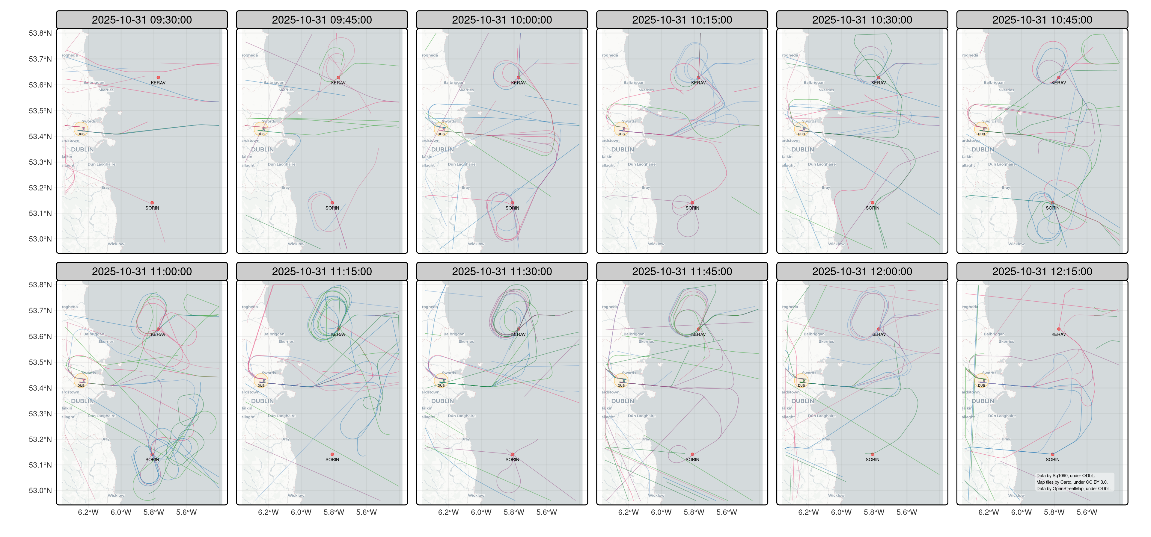
Figure 3.1.1 Aircraft traffic at KERAV and SORIN holding fixes near Dublin Airport on 31 October, 2025.
3.2. Assumptions
At a technical level, this tutorial assumes familiarity with
Structured Query Language (SQL) and Common Table Expressions (CTEs) within PostgreSQL relational database system.
R programming language for statistical analysis.
3.3. Bin Flights by Time Interval
Sq1090 project decodes ADS-B messages into aircraft positions and stores the
data in the position database table. The table has time, aircraft ICAO
address, and aircraft location columns (see the Section 3
for details)
timeTime of receiving a raw message with aircraft location and altitude.
icaoICAO address of an aircraft. It is an integer number displayed as a hexadecimal number.
locationLocation and altitude of an aircraft. The positions are stored using WGS 84 coordinate system.
Query the position table to find flight timeline of each aircraft
within the geographical area covering KERAV and SORIN holding fixes and
Dublin Airport on October 31, 2025
1select
2    date_trunc('second', time) as tb_sec,
3    to_hex(icao) as icao,
4    st_centroid(st_collect(location)) as location
5from position
6where st_within(location, st_makeenvelope(-6.375, 52.96, -5.37, 53.8, 4326))
7    and time between '2025-10-31 09:30Z' and '2025-10-31 12:30Z'
8group by tb_sec, icao
The query
[2-4]extracts positions of each aircraft at one-second intervals, calculating average position if multiple data points exist within the same second[6]finds aircrafts within the geographical area using a PostGIS spatial index to optimise execution of the predicate function[7]filters the data leveraging TimescaleDB time index to optimise bucketing and finding aircraft positions based on the specified time interval
Having flight timeline, bin flights into 15-minute time intervals and identify track of each aircraft
1select
2    time_bucket('15 minutes', tb_sec) as tb,
3    icao,
4    st_astext(st_makeline(location order by tb_sec)) as track
5from timeline
6group by tb, icao
7having count(location) > 1
The query
[2-3]buckets positions of each aircraft into 15-minute intervals[4, 7]creates chronological sequence of aircraft positions; there needs to be at least one location
The final data query is
 1with timeline as (
 2    select
 3        date_trunc('second', time) as tb_sec,
 4        to_hex(icao) as icao,
 5        st_centroid(st_collect(location)) as location
 6    from position
 7    where st_within(location, st_makeenvelope(-6.375, 52.96, -5.37, 53.8, 4326))
 8        and time between '2025-10-31 09:30Z' and '2025-10-31 12:30Z'
 9    group by tb_sec, icao
10)
11-- bin flights into 15-minute intervals
12select
13    time_bucket('15 minutes', tb_sec) as tb,
14    icao,
15    st_astext(st_makeline(location order by tb_sec)) as track
16from timeline
17group by tb, icao
18having count(location) > 1
3.4. Read and Visualise Data
Sq1090 database can be queried with SQL by many applications and programming languages. This tutorial uses R programming language to read and visualise the data.
In R, use RPostgreSQL library to execute queries against Sq1090 database.
There are many options to visualise the data on a map in R. tmap is an R package for drawing thematic maps using grammar of graphics concept. It integrates with sf package, which in conjunction with dplyr library, enables creating and manipulating geographical data (simple features).
Additionally, use urltools library to pass database system parameters to the script developed in this tutorial.
Install the libraries in R language environment, for example using its
shell and install.packages function
$ R
> install.packages(c('RPostgreSQL', 'dplyr', 'tmap', 'sf', 'urltools'))
In R IDE or a text editor, create file with name traffic-on-hold.
We will populate the R script with commands to read aircraft positions from
database, visualise traffic on a map, and save it into a PDF file.
Import the libraries
1library(dplyr)
2library(RPostgreSQL)
3library(sf)
4library(tmap)
5library(urltools)
Parse database connection and output file arguments
1args = commandArgs(trailingOnly=T)
2db = url_parse(args[1])
3output = args[2]
Connect to Sq1090 database and execute SQL query (QUERY variable is the
query defined in previous section)
1pg_drv = dbDriver('PostgreSQL')
2conn = dbConnect(pg_drv, dbname=db$path, host=db$domain, port=db$port)
3data = dbGetQuery(conn, QUERY)
Define geographical features for Dublin Airport and KERAV and SORIN holding fixes
1airport.sf = (st_point(c(-6.27, 53.4285))
2              |> st_sfc(crs=4326)
3              |> st_buffer(dist=3000))
4
5data.hold = st_sf(name=c('SORIN', 'KERAV'),
6                  location=list(st_point(c(-5.806250, 53.141472)),
7                                st_point(c(-5.765917, 53.628528))) |> st_sfc(crs=4326))
Convert data read from database into data with geographical features
1data.track = st_sf(data |> mutate(track=st_as_sfc(track, crs=4326),
2                                  icao=factor(icao)))
Plot the aircraft traffic for each 15-minute time interval in the geographical area covering Dublin Airport and KERAV and SORIN holding fixes (see the Figure 3.1.1 in the introduction)
 1credits = c(rep('', 11),
 2            'Data by Sq1090, under ODbL.\nMap tiles by Carto, under CC BY 3.0.\nData by OpenStreetMap, under ODbL.')
 3p = (tm_basemap('CartoDB.Positron')
 4     + tm_graticules(alpha=0.1, labels.size=0.5)
 5     + tm_shape(airport.sf, bbox=data.track |> st_bbox())
 6     + tm_sf(col='orange', col_alpha=0.5, fill='orange', fill_alpha=0.1)
 7     + tm_text('DUB', size=0.3, ymod=-1.25)
 8     + tm_shape(data.hold)
 9     + tm_dots('location', fill='red', fill_alpha=0.5)
10     + tm_text('name', size=0.4, ymod=-1)
11     + tm_shape(data.track)
12     + tm_sf(col='icao', col_alpha=0.5, col.legend=tm_legend_hide())
13     + tm_facets(by='tb', ncol=6)
14     + tm_layout(panel.labels=c(sprintf('%s', unique(data$tb))))
15     + tm_credits(credits,
16                  position=c('right', 'bottom'),
17                  size=0.3,
18                  bg=T,
19                  bg.color='white',
20                  bg.alpha=0.5))
21
22tmap_save(p, file=output, width=3840, asp=0, unit='px')
Execute the script to create the plot in PDF format
Rscript traffic-on-hold postgresql://localhost:5432/sq1090 traffic-on-hold.pdf
3.5. Conclusions
Sq1090 decodes ADS-B messages into aircraft position data.
The position data is stored in Sq1090 database position table.
Query the table to determine flight timeline of each aircraft within
a geographical area.
In this tutorial, we have implemented the R script to visualise aircraft traffic at KERAV and SORIN holding fixes near Dublin Airport.
The source code of the script can be found in Sq1090 project repository
You can study Sq1090 project data model by reading its reference documentation, the Section 3.